
Paul Park: Current Research
This page is meant to serve as introductory material for mixing with PWIs. Figures and videos for this page were all generated through MATLAB. For more details, look out for the paper to be published on this subject.
What is a PWI?
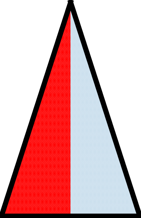
Generally speaking, a piecewise isometry (PWI) breaks a given object into a number of pieces and reassembles them into the same shape of the original object, but not in the same orientation. A PWI on an isosceles triangle is a classic example.
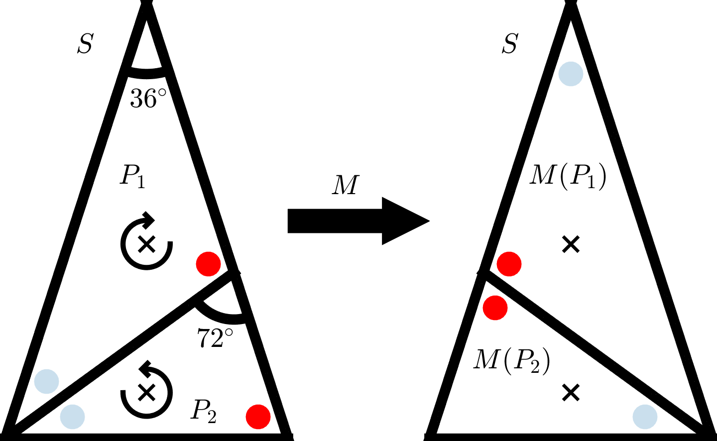 |
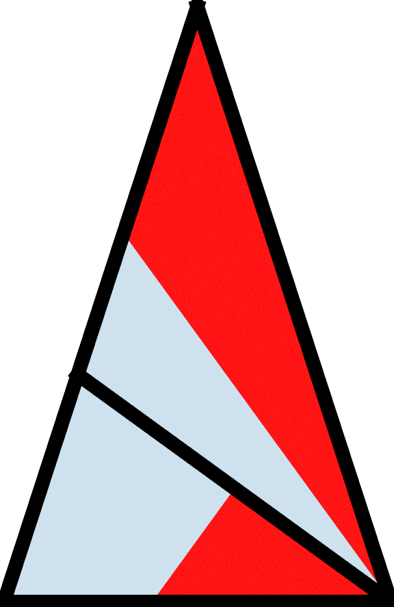
| An isosceles triangle is divided into 2 subtriangles which are also isosceles triangles. Each subtriangle is rotated accordingly such that the 2 form another large isosceles triangle |
Mixing with PWI
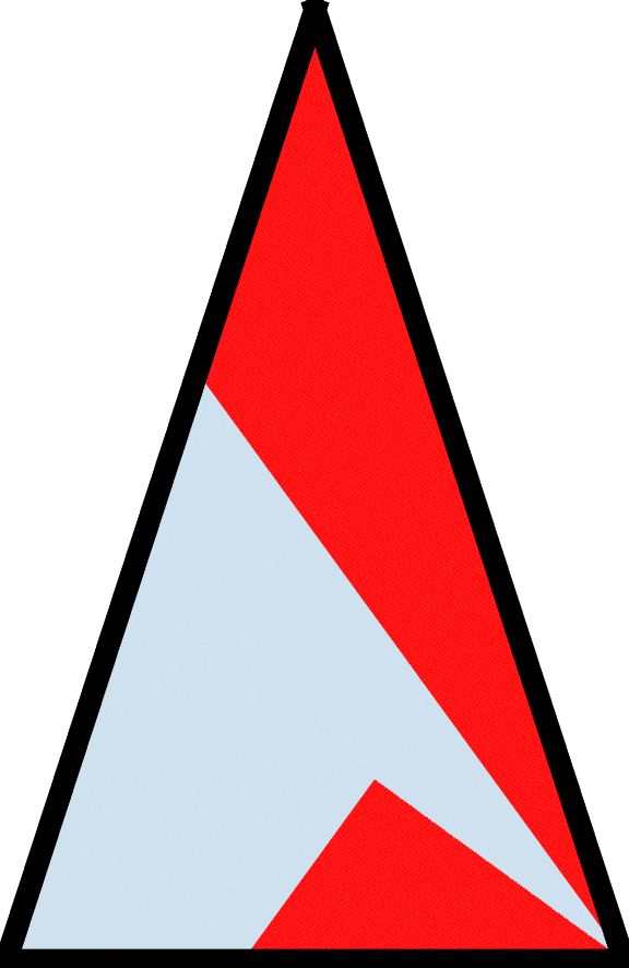
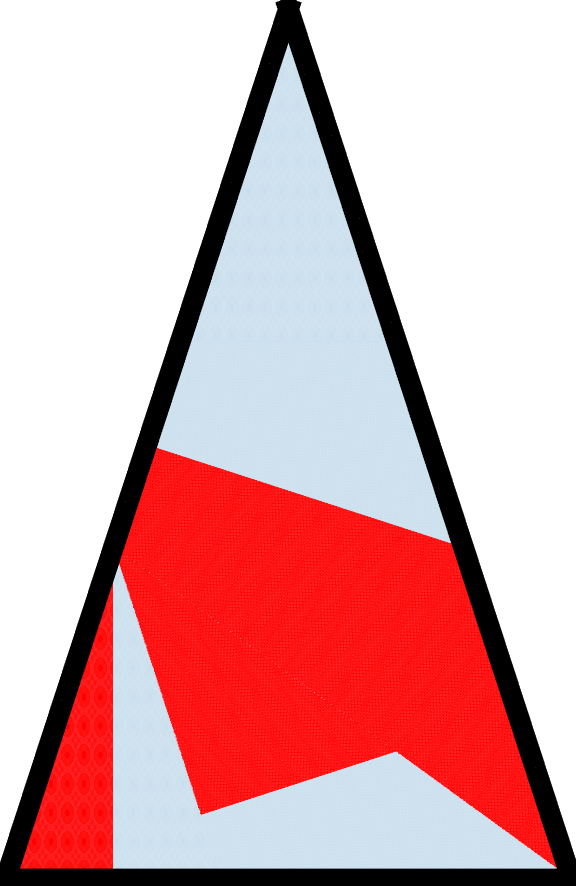
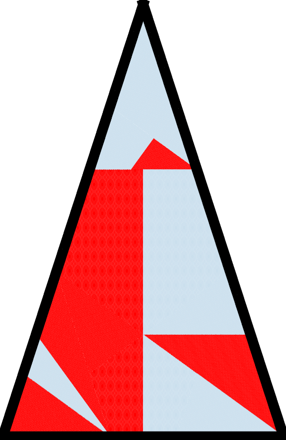
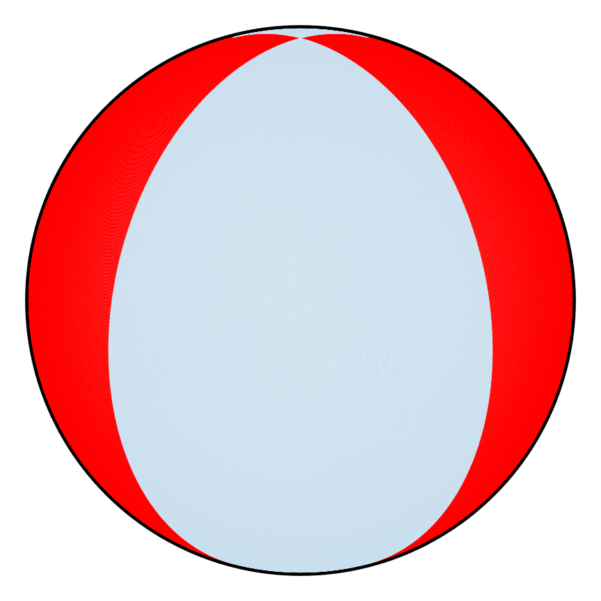
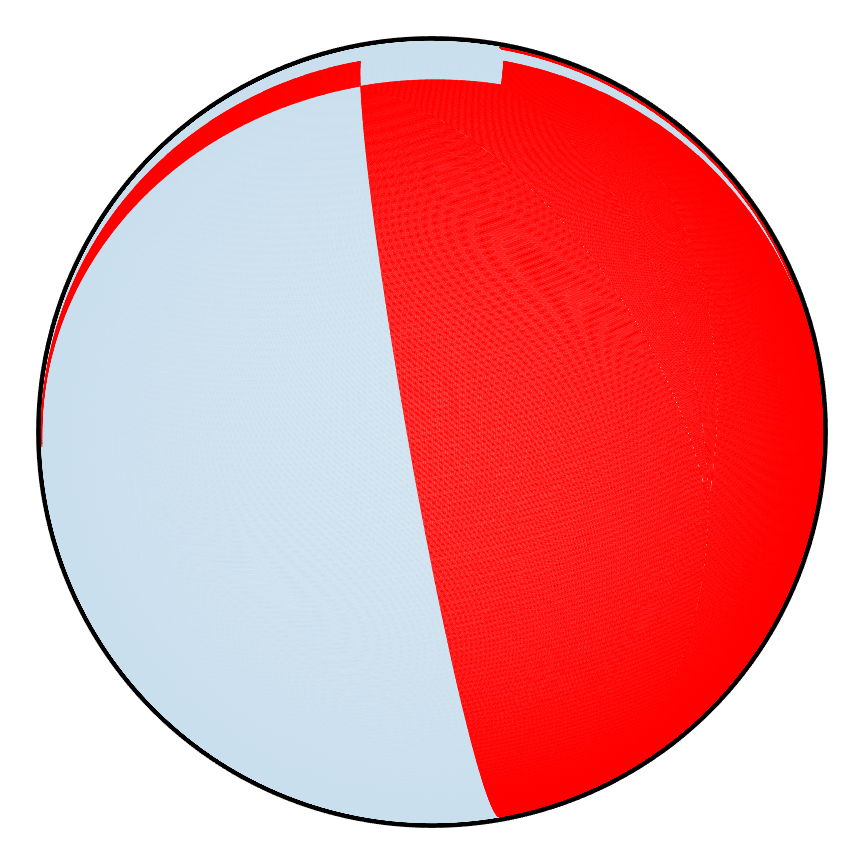
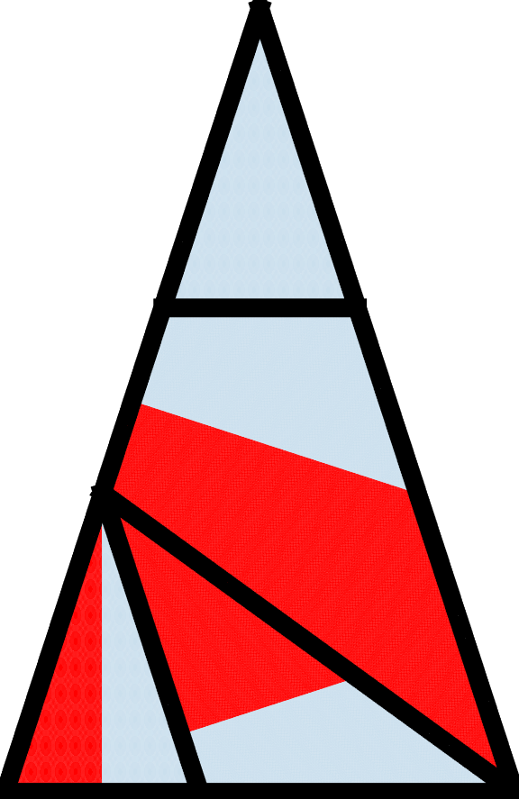
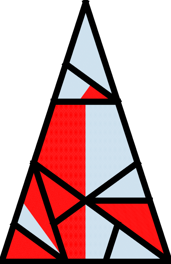
Imagine now that this operation is repeated for m iterations. The following figure shows what would happen if half of the isosceles triangle were red and the other half were blue initially.
 |
 |
 |
 |
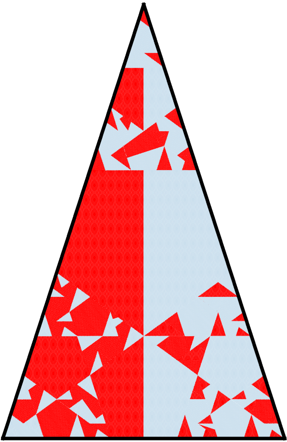 |
| m=0 | m=1 | m=2 | m=5 | m=60 |
At least with this example, it seems that mixing would be possible. The isosceles triangle however, is rather restrictive as a geometry in terms of the different types of PWI operations that can be applied to it. The hemispherical shell offers a more rich example in this case since it will allow us to compare mixing results based on the type of PWI applied to it. The video shows from left to right a 3D view, front view, and bottom view of a hemispherical shell going through a PWI transformation.
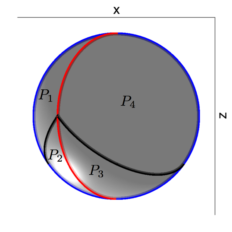
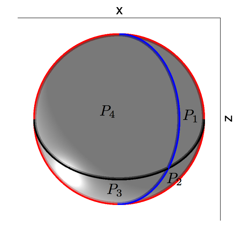
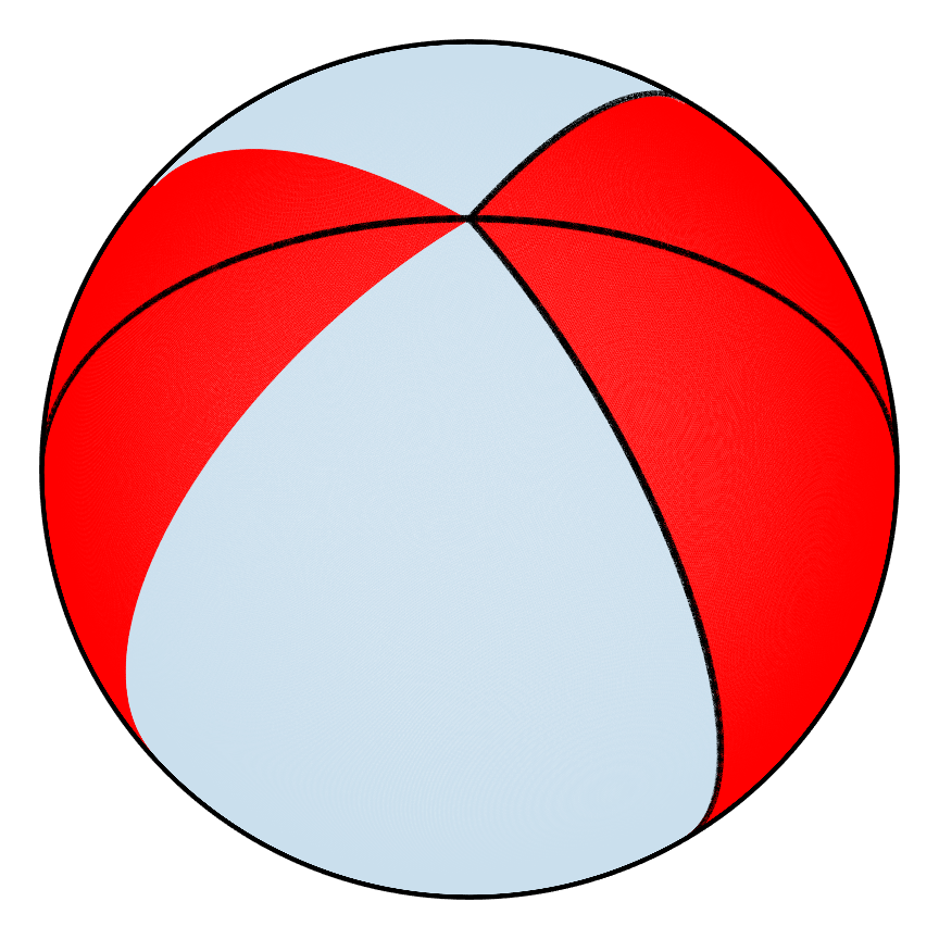
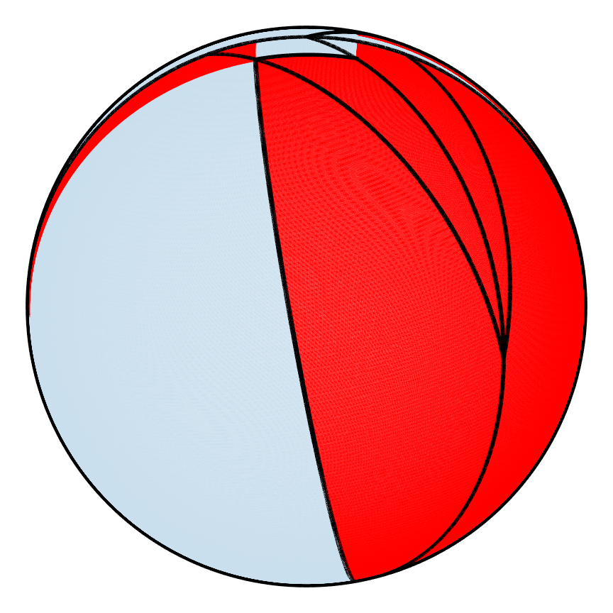
Notice in the video that there are two axes of rotation (z and x). After a rotation about the z axis, a portion of the shell that is above y=0 is cut from the rest and rotated over to get a new shell. The same goes for the x axis rotation that follows. Unlike the isosceles triangle which only had one kind of PWI, the hemispherical shell as shown in the video can have an infinite number of PWIs depending how much rotation occurs on each axis before the cut and rotation. The figure below shows the state of the shell (bottom view) after each rotation. The arcs drawn across the shell in red and black for the initial state indicate how the shell will be broken into four pieces that are rearranged again.
 |
 |
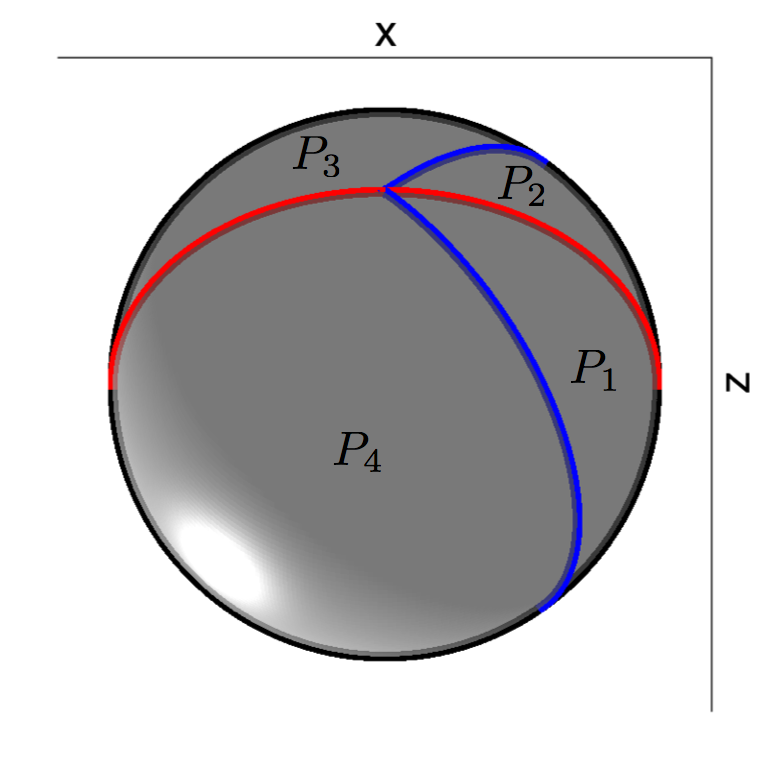 |
| Initial state | After z axis rotation | After x axis rotation |
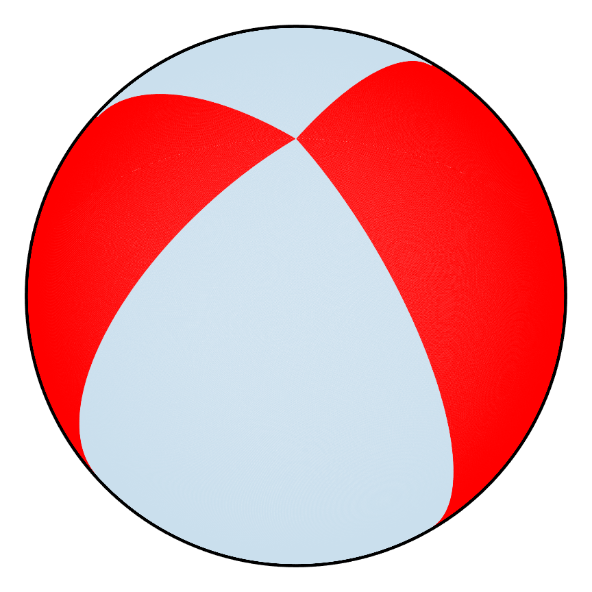
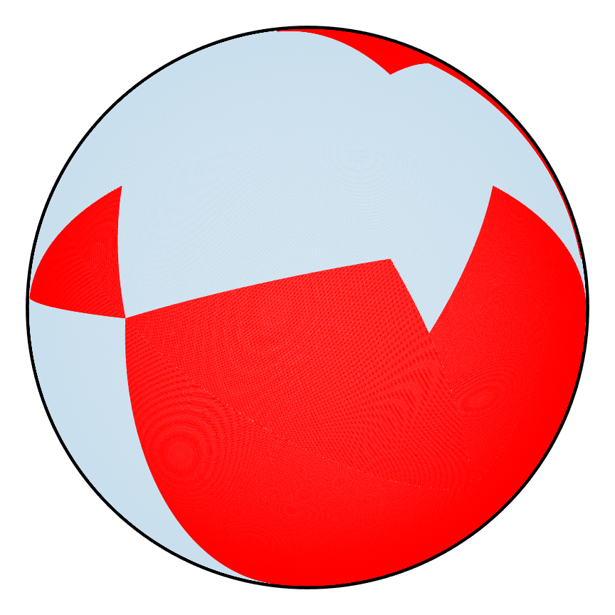
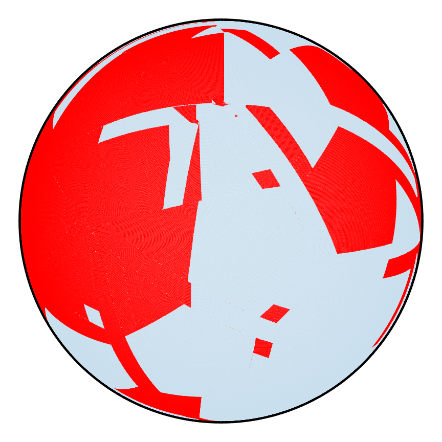
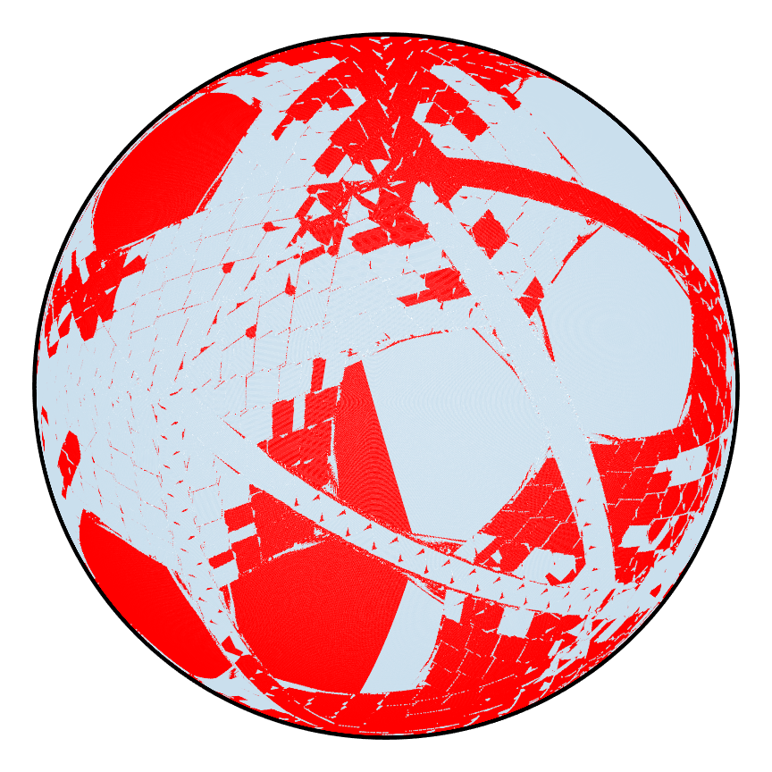
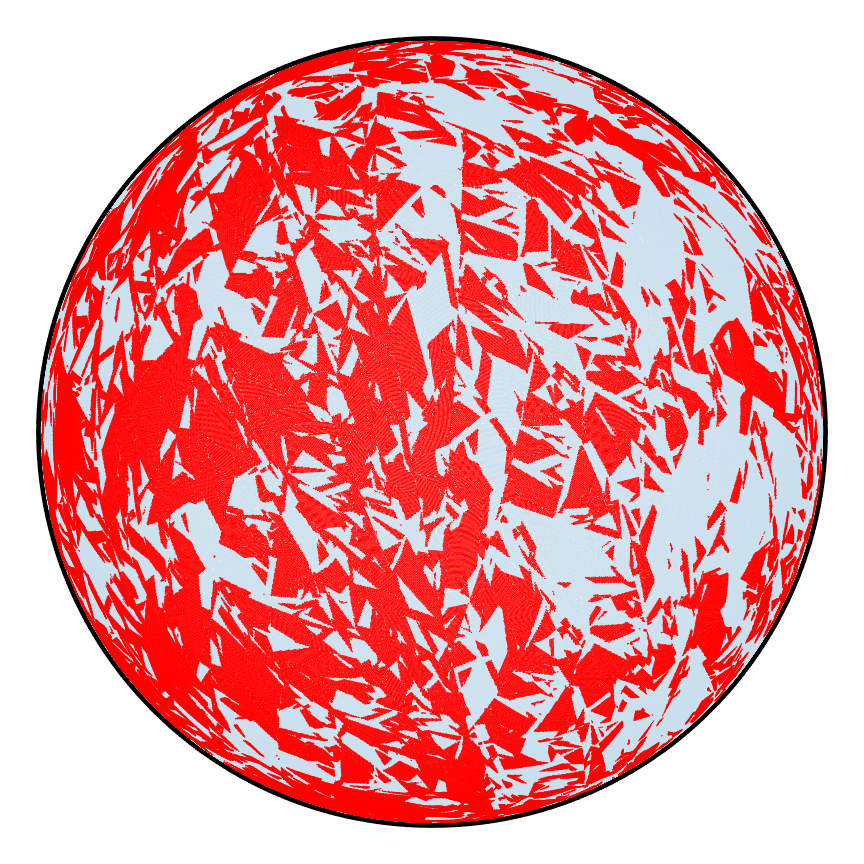
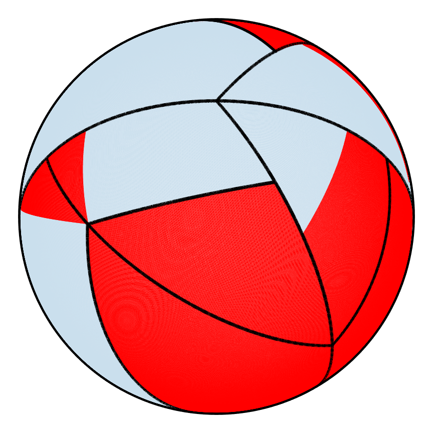
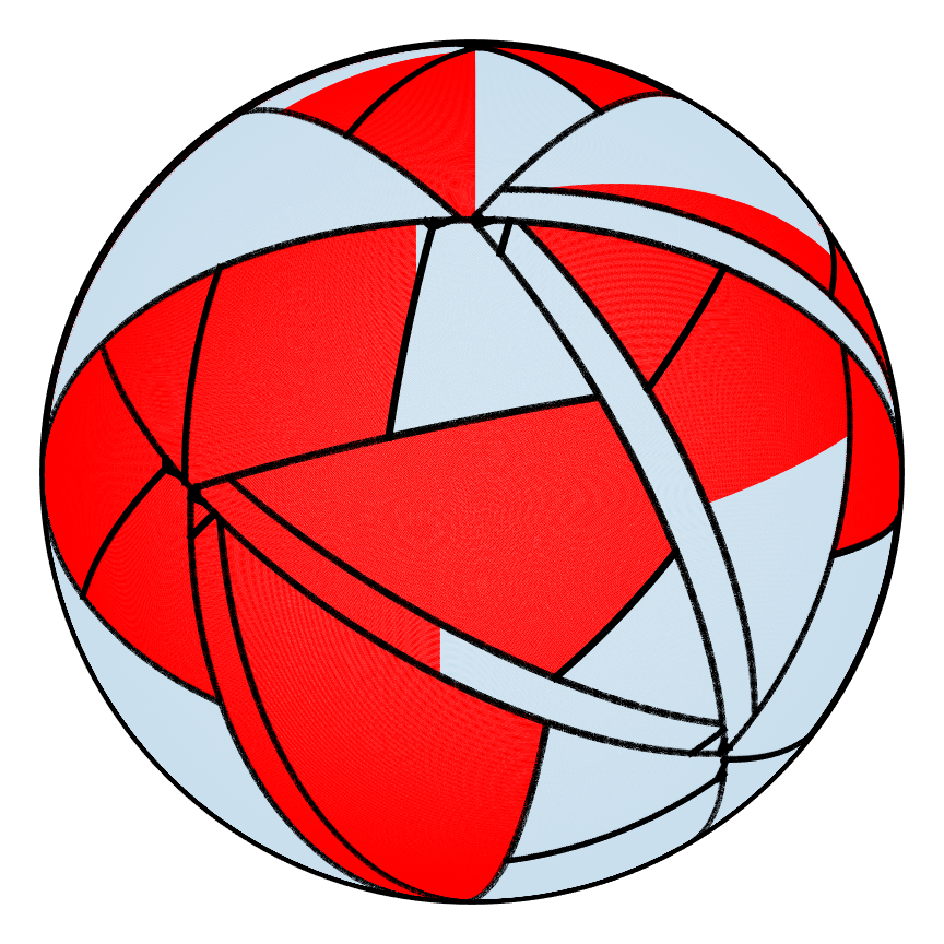
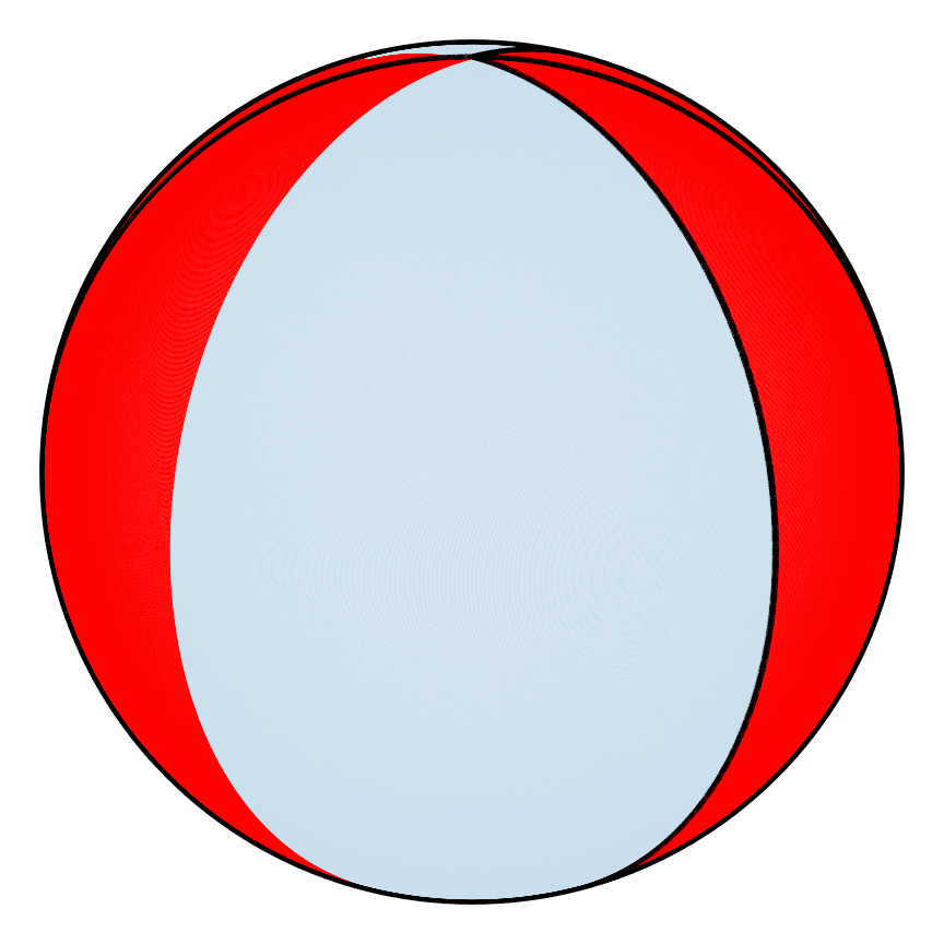
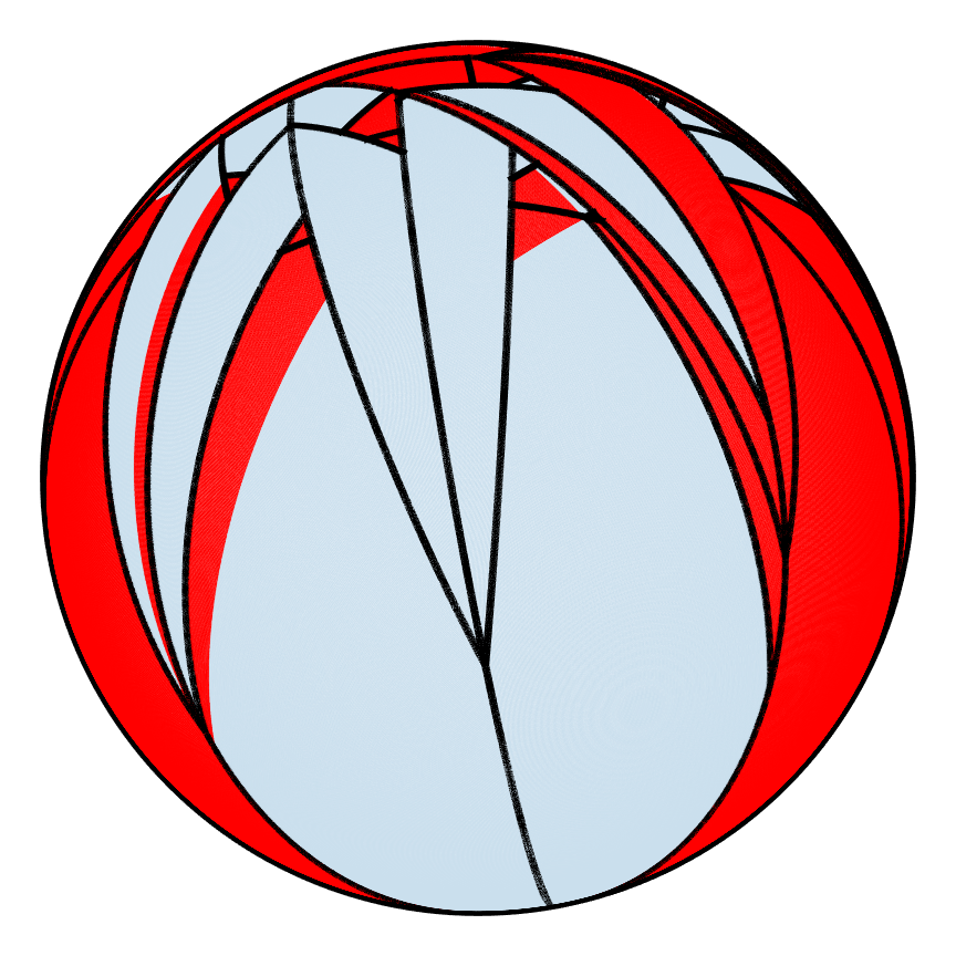
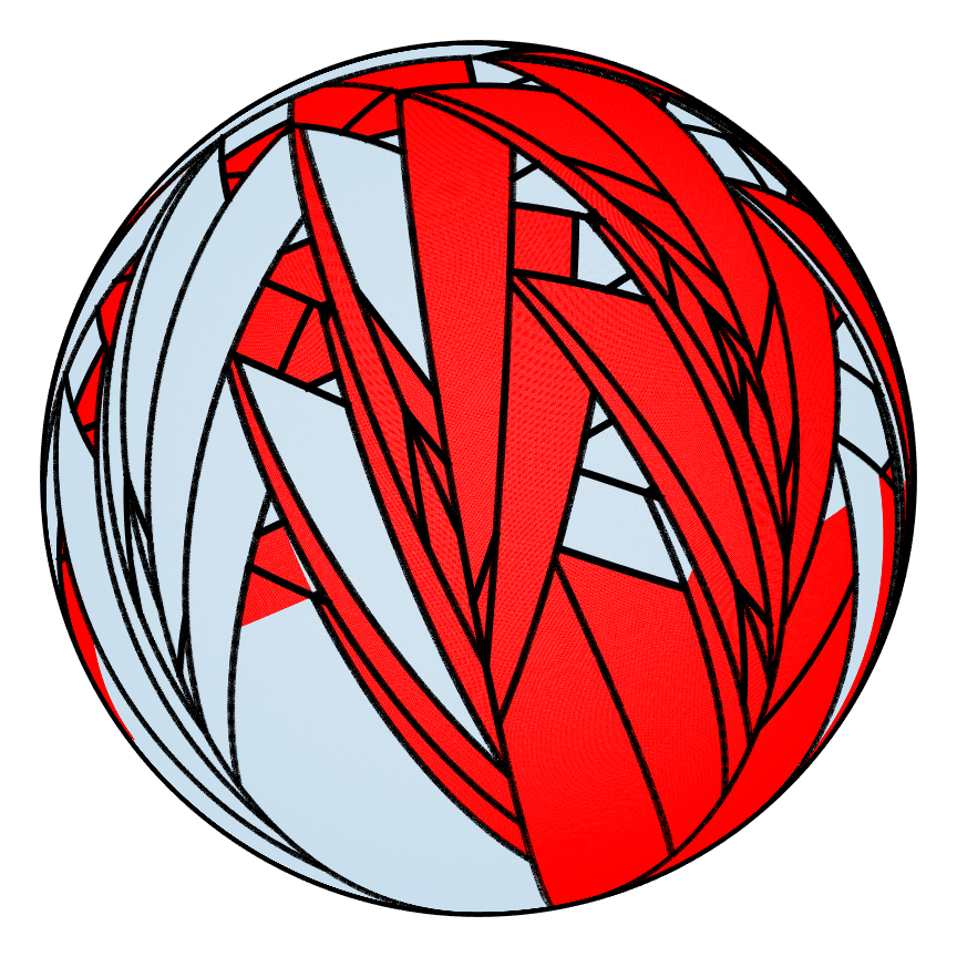
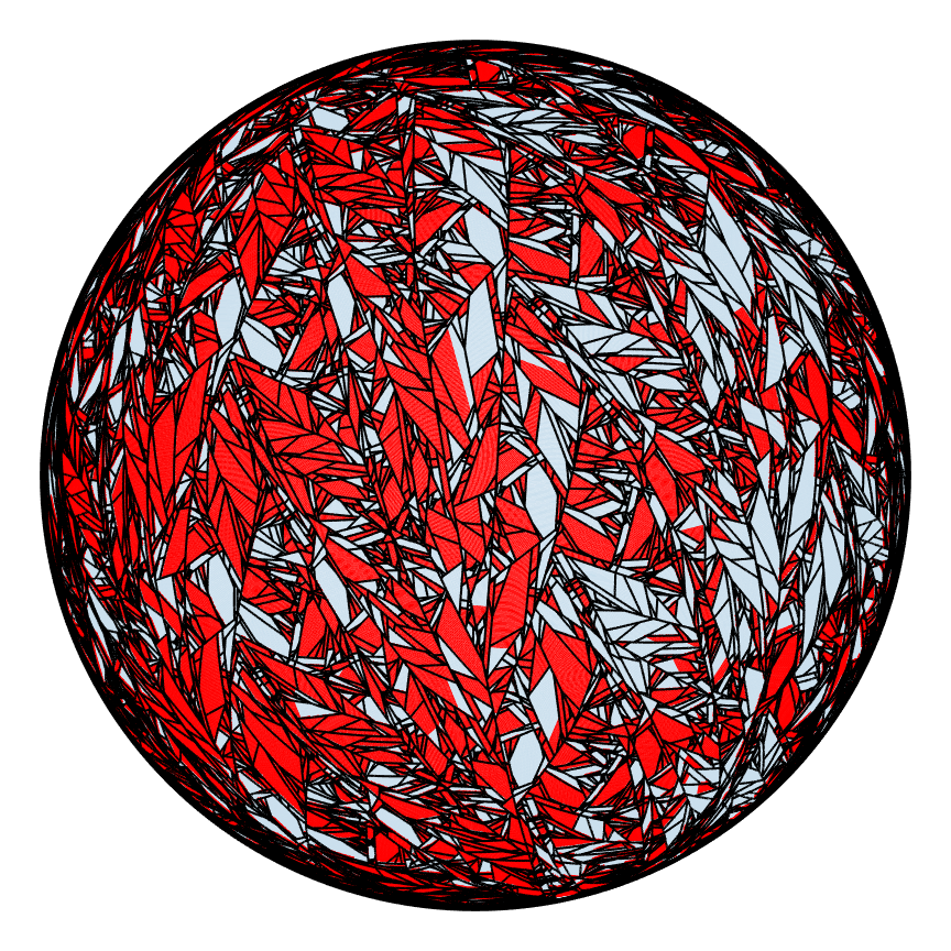
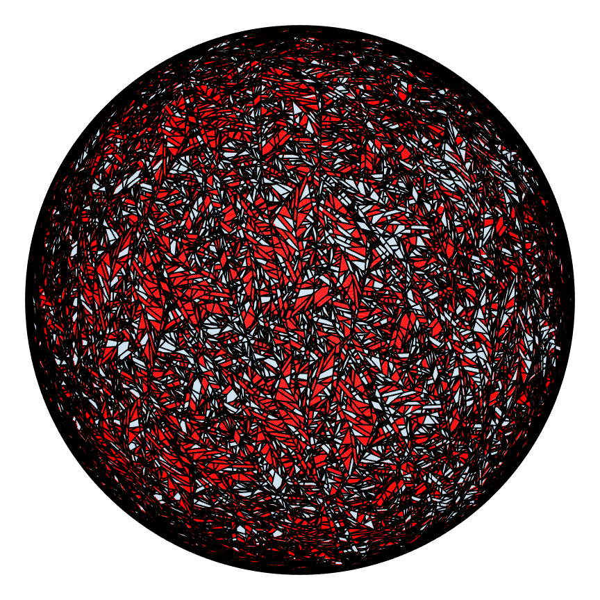
A set of z and x axis rotation counts as one iteration, and the process can be repeated just like the PWI on the isosceles triangle. Below is an example of a PWI on the hemispherical shell (bottom view) leading to poor mixing on the top row and good mixing on the bottom row.
| Poor |  |
 |
 |
 |
 |
 |
 |
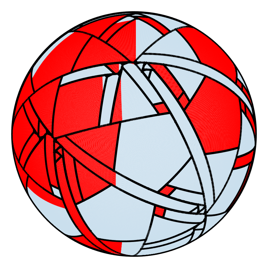
| Good | 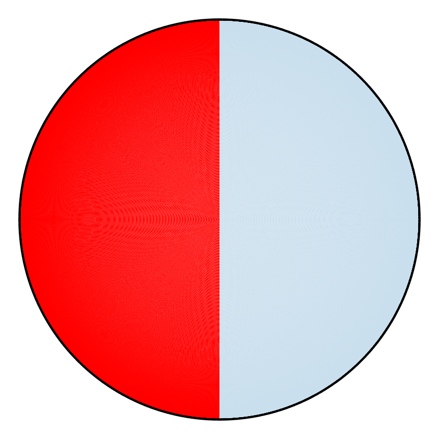 |
 |
 |
 |
 |
 |
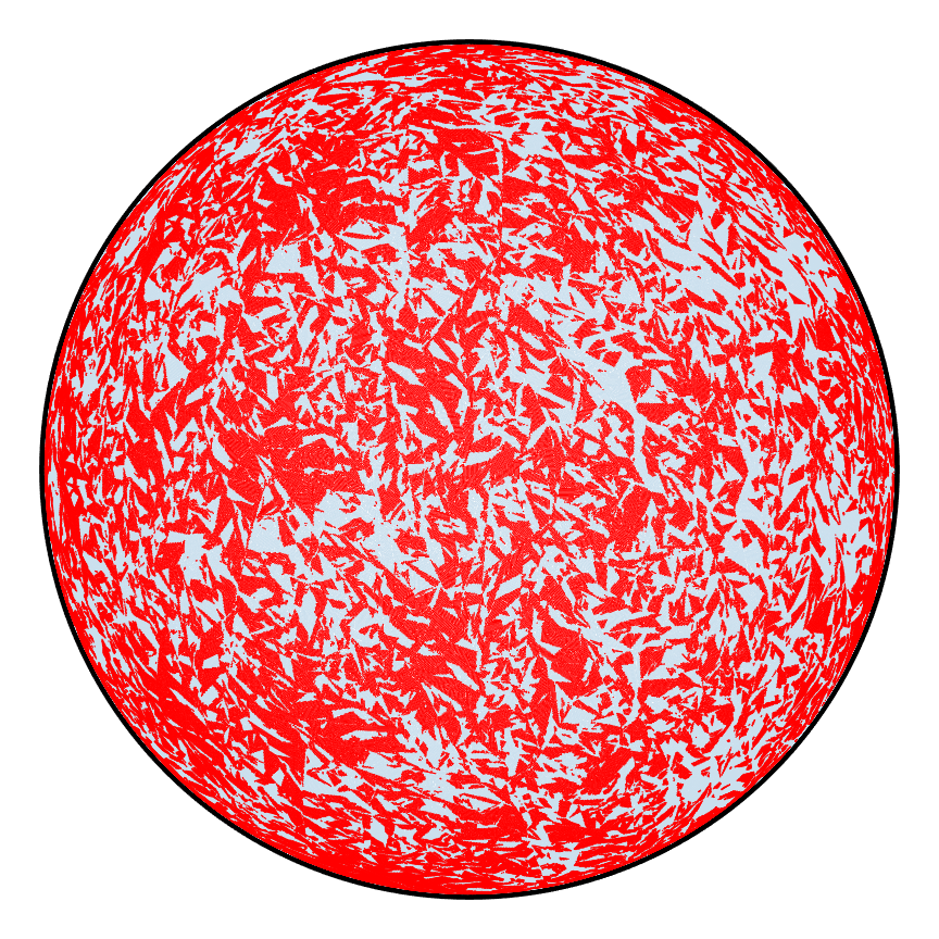 |
| m=0 | m=1 | m=2 | m=5 | m=10 | m=90 | m=180 |
Without going into the specifics of how to measure mixing, it is visually apparent that depending on the PWI, one could either get poor or good mixing, and we want to understand why that is case.
Time Maps
Perhaps one of the biggest challenges surrounding the study of mixing in general is the complication that arises from the dependence on the initial condition. Even though the mixing examples shown earlier involve two colors each occupying half of the domain, there is no reason why mixing should ever start that way. Nor should the mixing always only involve two different species. Our choice of the initial state was for all intents and purposes, quite arbitrary. A more fundamental understanding is desired, and one possible method for achieving this is to figure out the underlying dynamics for each PWI.
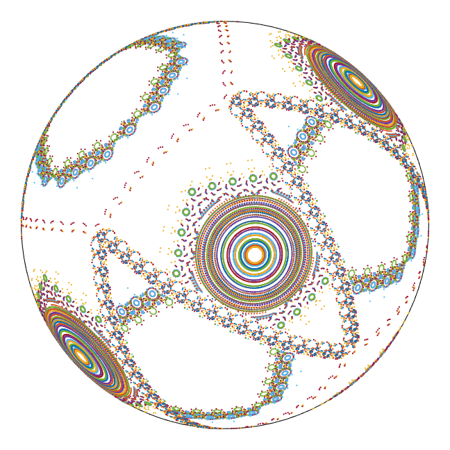
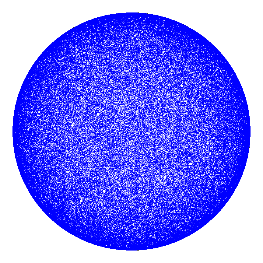
In all of the mixing examples, the entire domain was seeded with points (on the order of hundreds of thousands) such that collectively they seemed like a continuous whole, but this is not necessarily the best way to understand the characteristic behavior of the given PWI. At best, one can only conclude whether a given example ends up mixing well or not without being able to explain why. A common approach in such cases is to select a set of points (that is not the entire domain) and record where they go from one iteration to the next. The resulting plot is what is known as a time map for the set of points chosen. The figure below shows the time maps for the two PWIs for points (Set 1) that were selected on a diagonal arc crossing the hemispherical shell which were followed for 500 iterations where different colors correspond to the trajectory of different points.
| Poor | 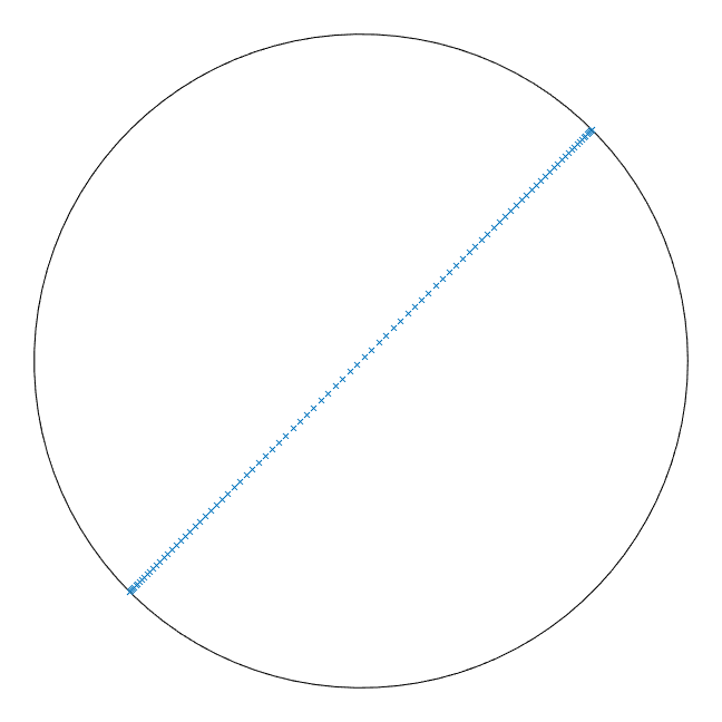 |
 |
| Good | |
 |
| Set 1 | Time Map |
The two time maps look quite different, and the trajetories for the points chosen can be used to infer certain characterisitics for each PWI. The time map for poor mixing shows many nested circular trajectories as well as chains of such circular trajectories. Such behavior is called elliptic, and is commonly associated with non-mixing regions, which explains why the first PWI mixes poorly. Another important feature is the fact that some of the regions on the shell are empty, meaning that the points that were chosen were not able penetrate those regions, implying the existence of barriers to motion, which also have negative implications for mixing. The time map for the second PWI on the other hand fills the entire domain. There are no elliptic regions, and there do not seem to be any barriers to motion either.
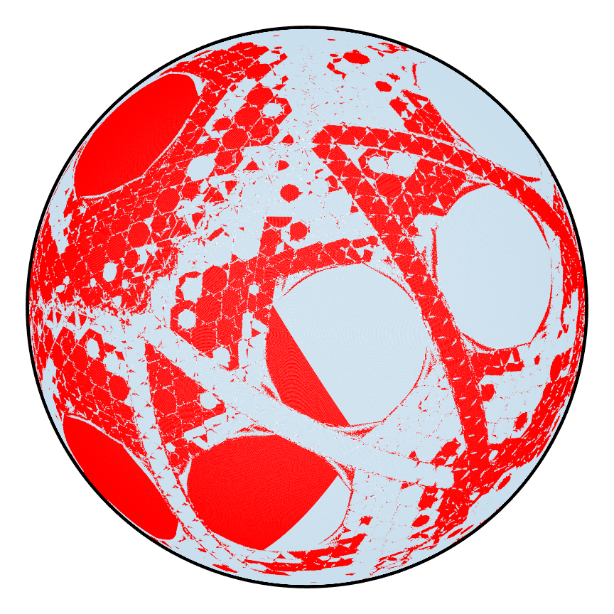
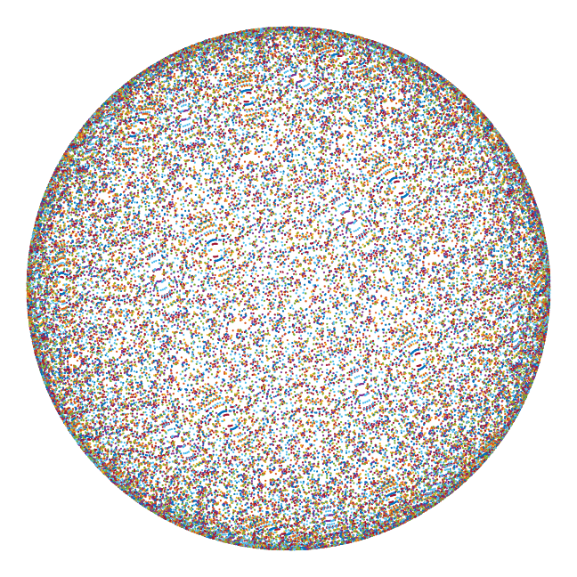
Again, the choice for the set of points followed was rather arbitrary, but the resulting trajectories turned out to be meaningful. A systematic approach that works for all PWIs would be more desirable, and for the sake of exploring, let's try a set of points (Set 2) that outline the borders of the different pieces of the shell for each PWI as shown in the figure below and track them for 1000 iterations. Because we are following so many points, it is not as useful to color code each one so the time maps are shown in blue. The reason for a large number of iterations is because time maps are generally used to approximate what the dynamics look like in the limit of infinite repetitions i.e. to obtain an asymptotic picture of the dynamics. If some pattern were to result from this, it could be used to interpret the dynamics as was done before, and as will be done for this example.
| Poor | 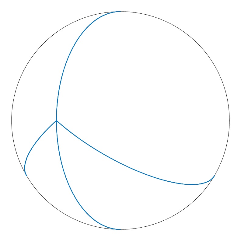 |
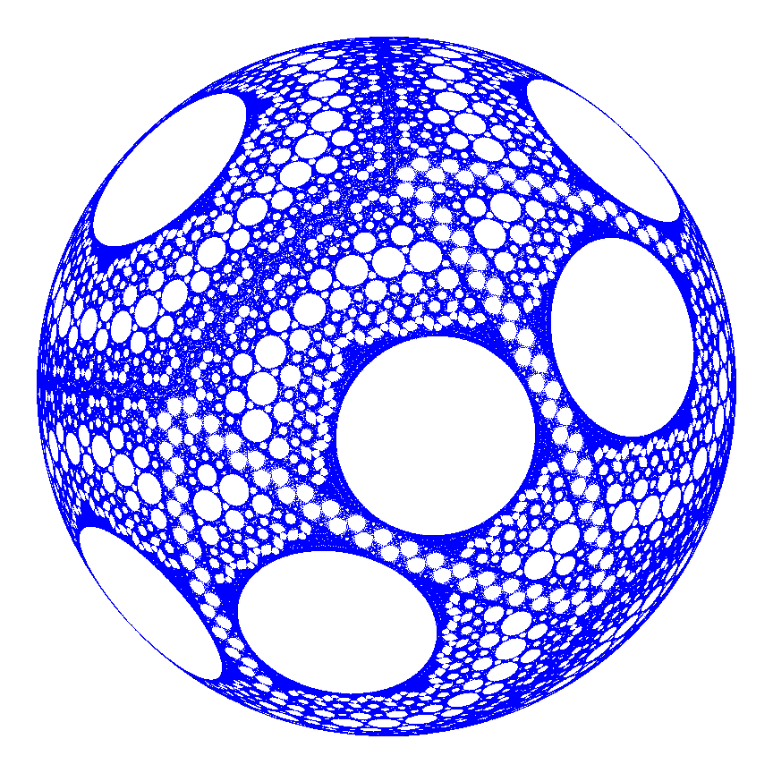 |
| Good | 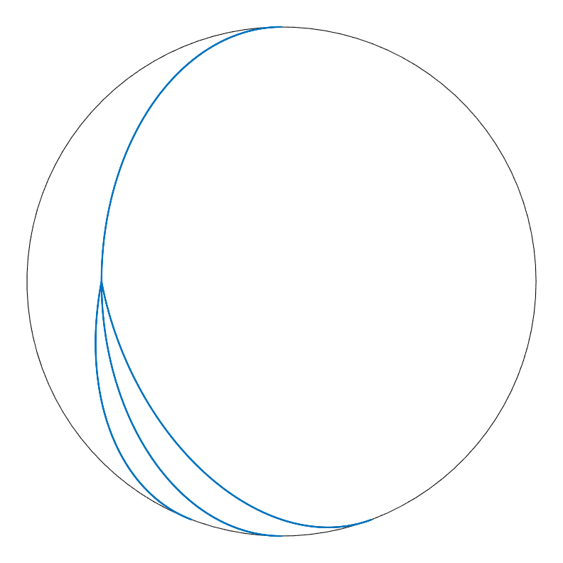 |
 |
| Set 2 | Time Map |
Again, the difference in patterns is quite striking, but what is also noticeable is the difference between the first set of time maps and the second set of time maps. The current time map for the first PWI (poor) seems more "complete" than the first one that was generated. There are still circular empty spaces, but one could hypothesize from previous results that all of these spaces might correspond to elliptic/non-mixing regions from visual inspection. Qualitatively, the time map for the second PWI (good) does not seem all that different from before. What is perhaps most interesting about these time maps is the idea that non-mixing regions can be identified ahead of time for any PWI before any mixing is attempted. One can imagine that this would be a useful factor to consider in any mixing application. The question then becomes how do we prove that the empty spaces in the second set of time maps actually correspond to non-mixing regions for all PWIs regardless of geometry?
Partitions for a PWI
Mixing can be considered largely as a two-step process consisting of a separation of the material followed by a joining of the material. In order to mix in a fixed domain or geometry, it is necessary for materials to separate to have any hope for mixing. How the material is joined or reassembled again is also important, but the second step cannot happen without a proper first step. In the context of PWIs, where the domain is broken apart before being reassembled, it might be worthwhile to consider how the domain is partitioned after each iteration as shown below for the isosceles triangle.
 |
 |
 |
 |
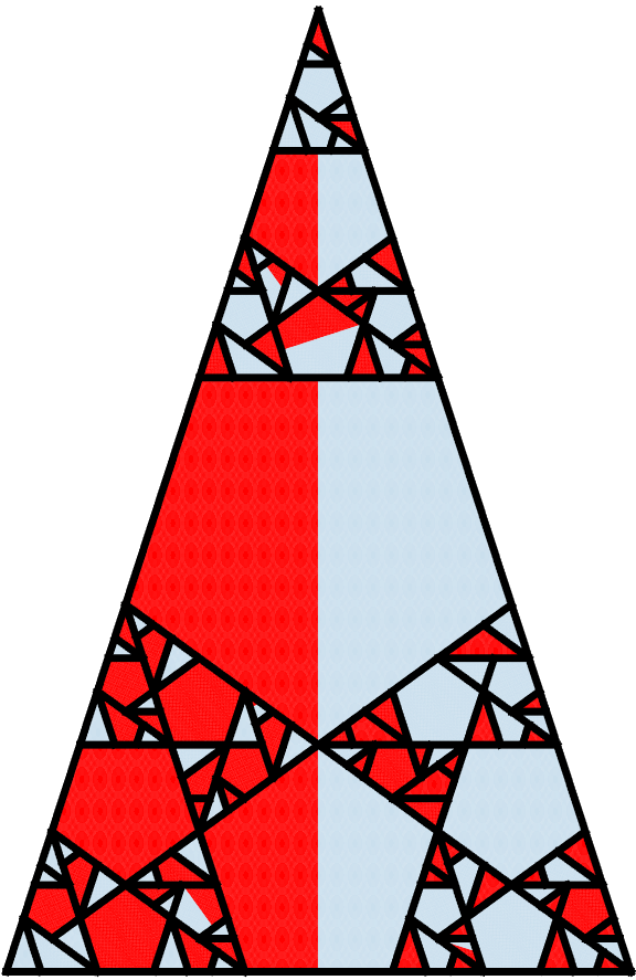 |
| m=0 | m=1 | m=2 | m=5 | m=60 |
The current figure of the isosceles triangle is the same as the previous one with mixing, with the addition of black lines in the interior indicating the borders of the different partitions. Notice the large pentagon in the center of the isosceles triangle for m=5, and the smaller pentagon below it. This feature remains the same even after m=60, and it would not be too hard to predict that such would be the case given the nature of this particular PWI. The large pentagon is always a part of the upper triangle, and the smaller pentagon is always a part of the lower triangle at every iteration. The colors in these regions always stick together, and are never broken apart; mixing will not happen in these regions.
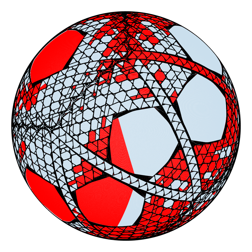
Partitions can also be tracked for the hemispherical shell as shown below. The first PWI after 180 iterations has many areas that have not broken apart whereas for the second PWI, the shell is partitioned so finely that the borders of the partitions cover up the shell, which explains why one PWI mixes better than the other.
| Poor | 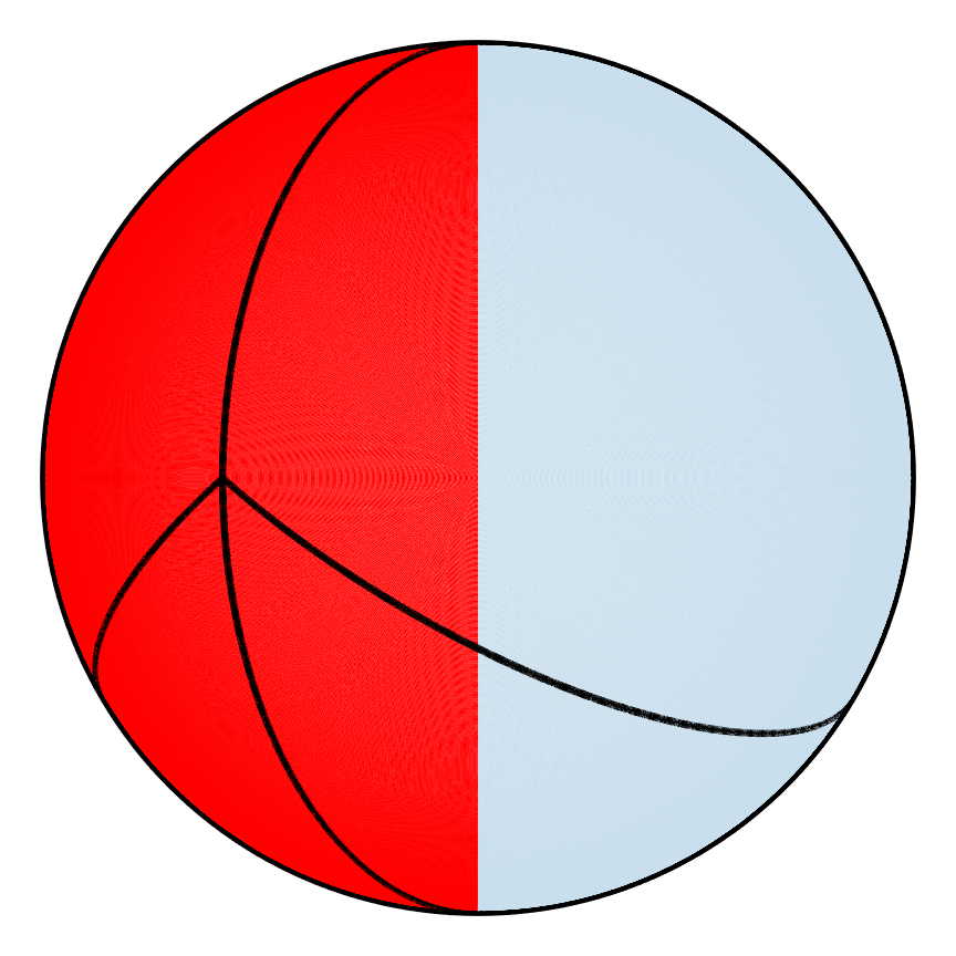 |
 |
 |
 |
 |
 |
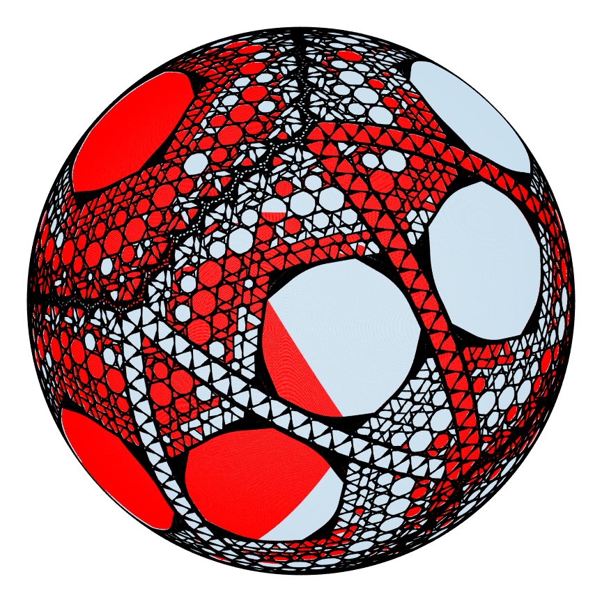 |
| Good | 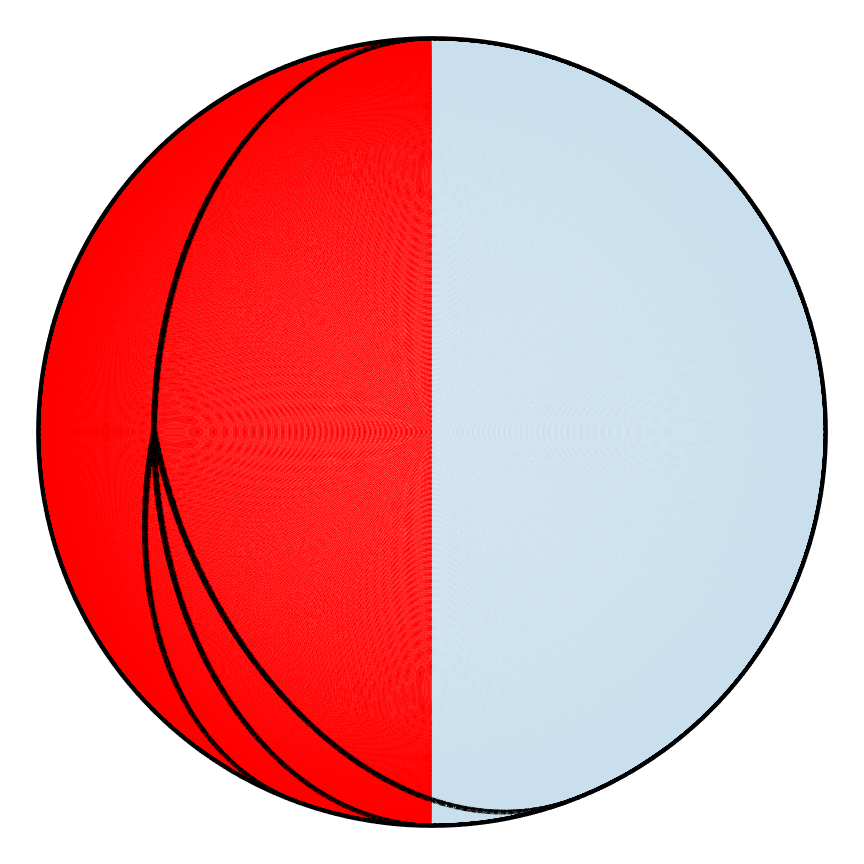 |
 |
 |
 |
 |
 |
 |
| m=0 | m=1 | m=2 | m=5 | m=10 | m=90 | m=180 |
Consider now the partitions after 180 iterations and the time maps from before. They look remarkably similar, and given the fact that the empty spaces in the partitions indicate areas that are not broken apart, and thus do not mix, it is reasonable to question whether the relationship between the partitions and time maps can shed light on the question of identifying non-mixing regions for PWIs.
| Poor | 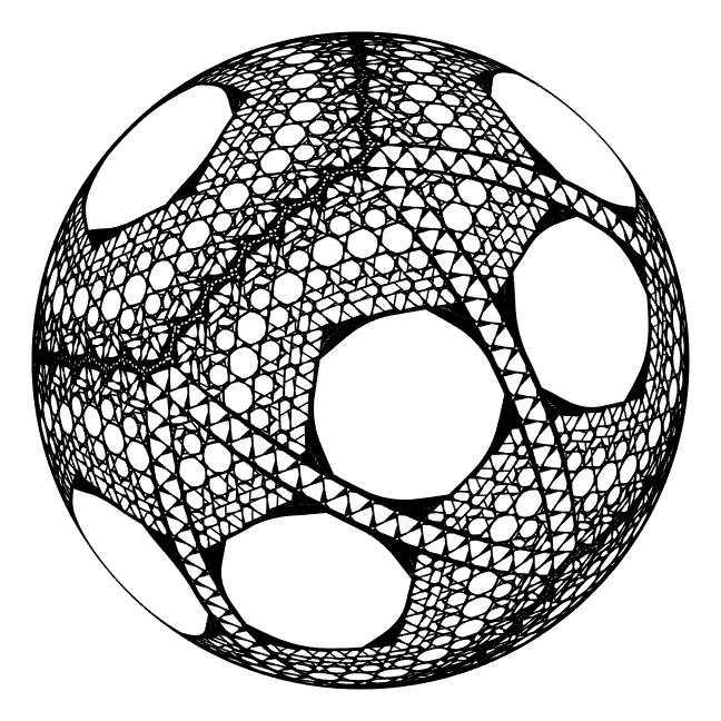 |
|
| Good | 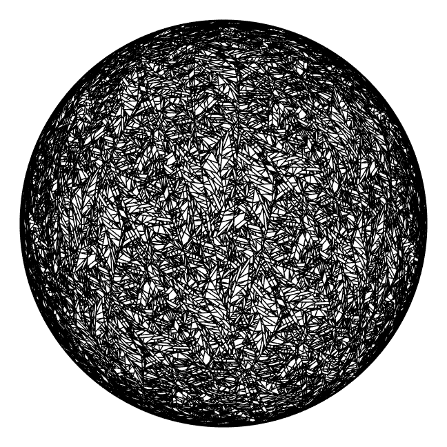 |
|
| Partitions after m=180 | E+ |
Next Step?
Much of this section has relied on visual observations and to a lesser extent, some heuristics to introduce the topic of mixing with PWIs. The figures shown below are all connected, and a more rigorous approach is necessary to clarify how they relate.
| Poor | |
|
|
|
| Good | |
|
|
|
| Mixing | Arbitrary Time Map | Partitions | Time Map, E+ |